- Why multireference — the limits of single-reference
- The active space CAS(n, m)
- A first CASSCF — H2(2,2)
- Reading the output — CI vector and occupations
- Several states at once — state-averaging
- Dynamic correlation — NEVPT2
- Spin-orbit coupling and magnetic properties
- Large systems — metal / ligand fragment merge
- Limits and what's next — DMRG
Why multireference — the limits of single-reference
HF, DFT, and CCSD(T) all assume that a single Slater determinant dominates. That holds for closed-shell organics and ordinary radicals. The moment two or more determinants carry comparable weight, the assumption collapses and the single-reference answer goes qualitatively wrong. The usual offenders are molecules midway through bond breaking, non-colinear magnetic states in transition-metal and lanthanide complexes, singlet diradicals, and the region around conical intersections.
The cleanest example is H2 dissociation. The curves below scan the H–H distance from 0.4 to 3.0 Å with RHF and CASSCF(2,2) — real calculations on ORCA 6.1.1, cc-pVDZ.
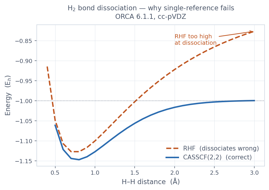
Near equilibrium both are fine, but as the bond stretches RHF runs away upward (−0.826 Eh at 3.0 Å). Closed-shell RHF keeps both electrons in the σ bonding orbital, so it cannot separate cleanly into two neutral H atoms — ionic terms are forced in. CASSCF adds the σ*2 configuration to the wavefunction and dissociates correctly to two H atoms (−1.0 Eh). Treating those two configurations, σ2 and σ*2, at the same time is the heart of multireference theory.
The active space CAS(n, m)
CASSCF solves for every electron configuration within an active space.
CAS(n, m) means a full CI of n electrons in m orbitals.
The active orbitals are the chemically important ones near the frontier — where the
multireference character lives. For H2 that is the σ·σ* pair → CAS(2,2); for a
transition metal it starts from all the metal d (or f) orbitals plus the key ligand orbitals.
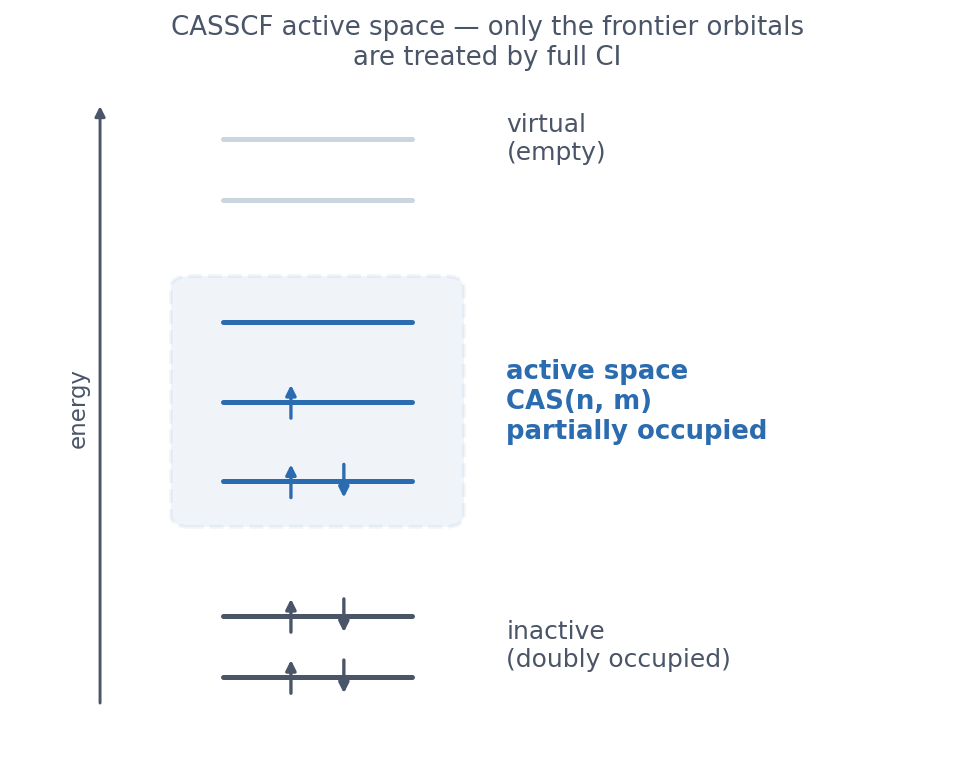
The result depends critically on the active space. Too small and it is inaccurate; too large and the cost explodes (the CAS dimension grows almost factorially with (n, m), so conventional CASSCF tops out near 14 active orbitals). Start from chemical intuition, then grow the active electrons / orbitals step by step and watch for convergence. The natural-orbital occupations (below) are a good guide.
A first CASSCF — H2(2,2)
The input behind the curves above. The bond is stretched to 1.5 Å so the multireference
character is obvious. The runnable file is in examples/05-casscf-h2/.
! CASSCF cc-pVDZ TightSCF

%casscf
   nel    2          # active electrons
   norb   2          # active orbitals (σ, σ*)
   mult   1          # multiplicity (singlet)
   nroots 1          # number of states
end

* xyz 0 1
  H   0.0   0.0   0.0
  H   0.0   0.0   1.50      # stretched bond → multireference
*
Reading the output — CI vector and occupations
Two lines of the real output tell the story. (Measured on ORCA 6.1.1.)
ROOT   0:  E=      -1.0561253815 Eh
      0.90503 [     0]: 20
      0.09497 [     2]: 02

N(occ)=  1.81007 0.18993

Final CASSCF energy       : -1.056125382 Eh
The CI vector writes the wavefunction as a sum of configurations.
[0]: 20 is two electrons in σ and zero in σ* (weight 0.905); [2]: 02
is both promoted to σ* (weight 0.095). A single-reference method would put ~100 % on the
first; the fact that the doubly-excited configuration carries 9.5 % is the
multireference character. Stretch the bond further and the two weights approach 50:50 (a
perfect diradical).
N(occ) is the natural-orbital occupation: 1.81 for σ, 0.19 for σ* — away from the single-reference 2.00 / 0.00. That departure from integer occupation is the key diagnostic. Rule of thumb: an orbital with occupation roughly between 0.1 and 1.9 belongs in the active space.
Several states at once — state-averaging
For excited states, or when several states sit nearly degenerate (common in transition
metals and lanthanides), optimising orbitals for one state biases the result.
State-averaged CASSCF averages the orbitals over several roots, giving one
common orbital set that favours no single state. Raise nroots, and split into
multiplicity blocks if needed.
%casscf
   nel    6
   norb   5
   mult   3, 1      # triplet and singlet blocks
   nroots 5, 5      # average 5 roots in each block
end
Dynamic correlation — NEVPT2
CASSCF captures static correlation (the near-degeneracy) but misses the
rest, the dynamic correlation. NEVPT2 adds it
perturbatively on top, and unlike CASPT2 it is free of intruder-state problems. Add one
PTMethod line to the %casscf block.
%casscf
   nel    2
   norb   2
   mult   1
   nroots 1
   PTMethod sc_nevpt2    # strongly-contracted NEVPT2
end
sc_nevpt2 (strongly contracted) is fast and robust; move to
fic_nevpt2 (fully internally contracted) for more accuracy.
Spin-orbit coupling and magnetic properties
For heavy elements (4d/5d transition metals, 4f lanthanides) spin-orbit coupling (SOC)
splits the states and sets the magnetic anisotropy. DoSOC true in the
rel block does second-order SOC via QDPT, and SINGLE_ANISO fits a
pseudospin Hamiltonian (g-tensor, zero-field splitting) — the standard tool for
single-molecule magnets (SMMs). Below is a single Dy(III) ion treated as CAS(9,7).
# Dy(III) 4f9 single ion — CASSCF(9,7) + NEVPT2 + SOC + anisotropy
! CASSCF def2-SVP DKH2 RIJCOSX def2/J TightSCF

%casscf
   nel      9                # Dy 4f9
   norb     7                # seven 4f orbitals
   mult     6, 4, 2          # sextet, quartet, doublet
   nroots   21, 224, 490     # Russell-Saunders terms
   PTMethod sc_nevpt2

   rel
      DoSOC   true           # 2nd-order SOC (QDPT)
   end

   SINGLE_ANISO true        # fit a pseudospin Hamiltonian
end

* xyz 3 6
   Dy   0.000   0.000   0.000
*
The H2 example on this page is a real run, but a heavy system like
Dy(III) needs a proper SARC basis, a large active space, and a long calculation,
so it was not run here. The SINGLE_ANISO values below (gz etc.)
are example values taken from the typical Ising-limit Dy(III) range; a
real complex gives different numbers.
g-FACTORS OF THE LOWEST DOUBLET:
   gx =   0.03
   gy =   0.05
   gz =  19.6        <-- large anisotropy → Ising-limit, SMM candidate
A large gz with gx, gy near zero is "Ising-limit
anisotropy", the first diagnostic of an SMM. The next step is POLY_ANISO,
which fits the exchange parameter J between metal centres to model polynuclear
behaviour (manual §9.27).
Large systems — metal / ligand fragment merge
Throwing a large transition-metal complex into CASSCF whole tends to give a stubborn SCF and a hard-to-choose active space. A common strategy is to split into fragments and merge: compute the metal centre and the ligand shell separately to get each fragment's orbitals, then merge the two orbital sets into the starting guess for the full system. CASSCF then begins with the metal d/f orbitals already cleanly separated.
ORCA ships a dedicated utility for this, orca_mergefrag. Run it with no
arguments and it prints its own usage.
orca_mergefrag FragmentA.gbw FragmentB.gbw Supermolecule.gbwProcedure — high-spin [Mn(H2O)]2+
Mn2+ is high-spin d5 (sextet), so all five d orbitals are singly occupied — the textbook case for a fragment merge. Compute the metal site and the water as separate fragments.
① Metal fragment fragMn.inp
! UHF def2-SVP
* xyz 2 6
  Mn  0.0  0.0  0.0
*
② Ligand fragment fragH2O.inp — at its supermolecule position, same basis
! UHF def2-SVP      # metal is UHF, so the ligand must be UHF too (HFTyp must match)
* xyz 0 1
  O   2.10  0.0  0.0
  H   2.65  0.76 0.0
  H   2.65 -0.76 0.0
*
③ Merge — run each fragment to get its .gbw, then
orca_mergefrag fragMn.gbw fragH2O.gbw superMn.gbwCheck the merge output (real run): atom counts, basis dimensions, and electron counts must all add up.
NAtoms(A)    =  1   NAtoms(B)    =  3   NAtoms(C)    =  4
Dimension(A) = 31   Dimension(B) = 24   Dimension(C) = 55     <- 31+24=55
NEl(A)       = 23   NEl(B)       = 10   NEl(C)       = 33     <- 23+10=33
Merging orbitals   ... done
Merging geometries ... done
Merging basis sets ... done
④ Supermolecule reads the merged guess for CASSCF — fragment A (Mn) comes first in the coordinates
! CASSCF def2-SVP MOREAD
%moinp "superMn.gbw"
%casscf
   nel  5
   norb 5
   mult 6
end
* xyz 2 6
  Mn  0.0  0.0  0.0
  O   2.10  0.0  0.0
  H   2.65  0.76 0.0
  H   2.65 -0.76 0.0
*
The merged guess drops the five Mn 3d orbitals straight into the active space. In the actual run the UHF step gave ⟨S²⟩ = 8.751 (sextet ideal 8.75, no spin contamination) and the CASSCF natural occupations came out N(occ) = 1.00 × 5 — a clean d5.
- Both fragments need the same HF type. If the metal is UHF, the
closed-shell ligand must be UHF too, or the merge stops with
HFTyp(A) must be HFTyp(B). - Fragment A's atoms come first in the supermolecule. The merge concatenates orbitals, geometry, and basis in A→B order, so list fragment A's atoms first and fragment B's after, in the same order.
- Same basis, same positions. Compute both fragments with the supermolecule basis, each at its position in the supermolecule geometry.
- The merged guess is not always better. Raw merged orbitals are not
energy-sorted, so the orbital rotation can diverge. As the tool suggests, run one SCF
on the merged guess to sort the orbitals before handing them to CASSCF, and if it still
thrashes use a robust optimiser such as
SuperCI_PT. For a simple system ORCA's default guess may already converge to the right d-occupation — this very example converges straight toN(occ)=1.0×5,E=−1225.0207 Ehfrom the default guess, making the merge unnecessary. Always check that the merge actually helps by comparing N(occ) and the energy against the default guess. It earns its keep on large, low-symmetry complexes where the default guess lands on the wrong d-occupation or spin state.
Replacing symmetry-equivalent metal sites with closed-shell analogues is a companion trick. In a Dy3 triangular cluster, swapping two of the three Dy for closed-shell Lu(III) exploits the C3 symmetry so only one site is treated explicitly.
Limits and what's next — DMRG
Conventional CASSCF runs out of memory once the active space passes 12–14 orbitals. From
there, ORCA 6's DMRG-CASSCF (%casscf actorbs DMRG) is the
standard and handles 30–40 active orbitals. For dynamic correlation beyond NEVPT2, move to
! MRCI+Q (multireference CI with the Davidson correction).
This chapter is an introduction, so it stops here. With the keywords in hand you can open manual §9 (CASSCF · NEVPT2) and §10 (MRCI) directly. To return to a single-reference method like CCSD(T), see 10 · DLPNO-CCSD(T).