Transition states · NEB

Three ways to locate a transition state

ORCA offers three broad approaches to finding a transition state (TS, saddle point):

NEB-TS — the recommended first attempt

NEB-TS combines the Nudged Elastic Band method with OptTS. Given only the reactant and product geometries it constructs a path between them, identifies the highest point, and then refines it to a true saddle point.

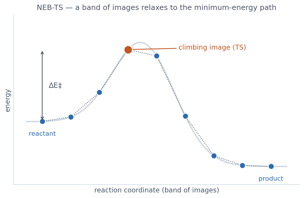
The example below is the intramolecular proton transfer in acetic acid (manual section 6.3.16):

# reactant.inp — start from the reactant geometry
! XTB NEB-TS

%neb
   neb_end_xyzfile "product.xyz"    # the product geometry
end

* xyz 0 1
  C    0.416   0.039  -0.014
  C    0.042   0.012   1.440
  O    1.524   0.177  -0.454
  O   -0.654  -0.128  -0.804
  H   -0.391  -0.126  -1.737
  H   -0.913   0.507   1.585
  H   -0.058  -1.026   1.751
  H    0.820   0.485   2.030
*

product.xyz must contain the coordinates of the same molecule in its product state (the proton on the other oxygen). The atom order has to match the reactant.

NEB-TS summarises its result like this:

---------------------------------------------------------------
                         PATH SUMMARY
---------------------------------------------------------------
Image Dist.(Ang.)    E(Eh)        dE(kcal/mol)     max(|Fp|)
  0     0.000     -14.45993           0.00          0.00011
  1     0.426     -14.44891           6.91          0.00092
  2     0.652     -14.42864          19.63          0.00084
  3     0.805     -14.41132          30.50          0.00075
  4     0.932     -14.40562          34.08          0.00057   <= CI (transition state)
  5     1.044     -14.41047          31.03          0.00057
  ...
  9     1.869     -14.45988           0.03          0.00013

The image marked "CI" (Climbing Image) is the converged transition state, and the dE column on that line is a first estimate of the activation energy in kcal/mol. NEB-TS then refines this point with OptTS, so the actual final number is the FINAL SINGLE POINT ENERGY at the end of the output file.

NEB variants

The variants documented in the manual trade cost against robustness:

OptTS — when you have a good initial guess

If you already have a geometry close to the TS together with an accurate Hessian, OptTS is the most efficient option. The Hessian must come from a frequency calculation at the same level of theory.

# Step 1: compute the Hessian at the initial guess geometry
! B3LYP D4 def2-SVP NumFreq
* xyzfile 0 1 ts_guess.xyz

$new_job

# Step 2: OptTS using the Hessian from step 1
! B3LYP D4 def2-SVP OptTS Freq
%geom
   InHess     Read
   InHessName "job1.hess"
   Calc_Hess  true          # recompute Hessian every 5 steps
   Recalc_Hess 5
end
* xyzfile 0 1

ScanTS — automate scan + TS search

When the reaction coordinate is a single bond length or angle, ScanTS is intuitive. ORCA scans the surface and, after passing the maximum, automatically uses that point as the initial guess for OptTS.

! B3LYP D4 def2-SVP ScanTS

%geom Scan
   B 2 5 = 2.5, 1.0, 16      # scan the 2-5 bond from 2.5 → 1.0 Å
end
end

* xyzfile 0 1 reactant.xyz

The moment the scan crosses its maximum, ORCA switches to OptTS automatically. The manual suggests computing a Hessian once at an intermediate scan point for better accuracy. To make ORCA finish the full scan before switching, add fullScan true.

IRC — validating the transition state

Once you have a TS, you must verify that it actually connects the intended reactant and product. The Intrinsic Reaction Coordinate (IRC) traces the steepest-descent path from the TS in both directions; it should arrive at the reactant on one side and the product on the other.

! B3LYP D4 def2-SVP IRC

%irc
   MaxIter   100
   PrintLevel 1
   Direction  both    # forward / backward / both
   InitHess   read
   Hess_Filename "ts.hess"
end

* xyzfile 0 1 ts.xyz

IRC can be chained with ! OptTS, ! ScanTS, ! NEB-TS, ! AnFreq, ! NumFreq, etc., so you can do "TS search → frequencies → IRC" in a single input file:

# NEB-TS → AnFreq → IRC all in one go
! B3LYP D4 def2-SVP NEB-TS AnFreq IRC

%neb
   neb_end_xyzfile "product.xyz"
end

* xyzfile 0 1 reactant.xyz

Recommended workflow

For a new reaction TS, this flow is recommended:

1. Optimise reactant and product with a cheap method (e.g. r2SCAN-3c or XTB).
2. XTB-NEB-TS to obtain a rough TS quickly (usually a few minutes).
3. DFT OptTS seeded with that geometry; include the Hessian.
4. AnFreq to confirm exactly one imaginary mode.
5. IRC in both directions to confirm the connection to reactant and product.
6. Single-point refinement: if needed, polish the final energy with DLPNO-CCSD(T)/cc-pVTZ or similar.

Following this workflow significantly improves the reliability of the result. Skipping IRC in particular risks publishing a "looks-like-a-TS-but-connects-the-wrong-reaction" false positive.