Why account for solvation
Gas-phase calculations describe a molecule in a vacuum. Real chemistry usually happens in solution, however, and a polar solvent can stabilise ions or molecules with large dipoles by anywhere from a few to several tens of kcal/mol. Ignoring solvation can put reaction equilibria, acid–base equilibria, and free-energy barriers far from experiment.
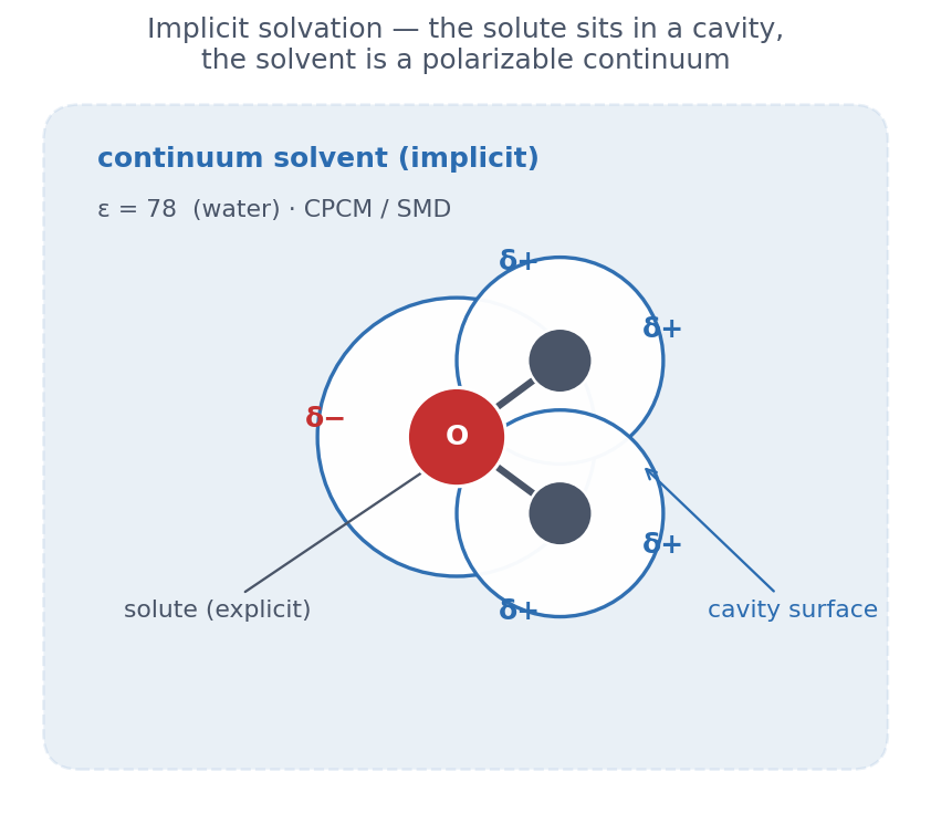
Available models — CPCM · SMD · ALPB
ORCA supports the following implicit-solvent models:
| Model | Keyword | Notes |
|---|---|---|
| C-PCM | CPCM(solvent) | Conductor-like polarisable continuum. Polarisation electrostatics only. Lightweight and robust. |
| SMD | CPCM(solvent) + %cpcm SMD true | Minnesota SMD. Adds non-electrostatic (cavity, dispersion, surface-tension) contributions. |
| ALPB | %cpcm ALPB true | Analytical Linearised PB. Often used with XTB. |
| openCOSMO-RS | Interface call | Post-processing for activity coefficients, log P, etc. |
This page focuses on the two you will use most often — CPCM and SMD. The manual activates both via the same keyword, but SMD also includes non-electrostatic terms (cavity formation, dispersion, surface tension) that make it more appropriate for free-energy comparisons.
Basic usage — one extra keyword
CPCM is activated by adding one keyword to the keyword line:
# Benzene optimisation in water (CPCM)
! B3LYP D4 def2-TZVP RIJCOSX def2/J Opt CPCM(water)

* xyzfile 0 1 benzene.xyz
In the formaldehyde example from the manual, the gas-phase n → π* excitation energy of 4.633 eV shifts to 4.857 eV in water with CPCM. The n-orbital is stabilised further in a hydrogen-bonding environment, so the excitation energy increases by 0.224 eV (~5 kcal/mol).
SMD — including the free-energy correction
Plain CPCM gives only the electrostatic free energy. For solvation free energies ΔGsolv or quantitative reaction equilibria, SMD — which includes the non-electrostatic correction — is more appropriate.
# Activate SMD — CPCM keyword + SMD true
! B3LYP D4 def2-TZVP RIJCOSX def2/J Opt Freq CPCM(water)

%cpcm
   SMD       true
   SMDSolvent "water"     # solvent must be repeated here
end

* xyzfile 0 1 mol.xyz
With SMD active, the output gains entries such as:
--------------------
SMD CDS free energy
--------------------
G-CDS (kcal/mol):              1.234567
...

----------------------------------------------------
SMD SOLVATION FREE ENERGY (CONTRIBUTIONS)
----------------------------------------------------
Total electrostatic    :     -8.456 kcal/mol
Total non-electrostatic:      1.235 kcal/mol
                         ===================
SMD ΔG_solv : -7.221 kcal/molSMD's parameters were originally calibrated for M05-2X/6-31G(d). In practice it works well with common DFT functionals (B3LYP, M06-2X, ωB97X-D, …) and a basis like def2-TZVP. Use the same method and basis as your gas-phase run, and compare ΔGsolv = G(soln) − G(gas) consistently.
Fine control — the %cpcm block
For precise control over the dielectric constant, refractive index and cavity shape, use the %cpcm block:
%cpcm
   Epsilon      80.4          # static dielectric constant (water)
   RefRac       1.33          # refractive index (for the dynamic response in TD-DFT)
   Rsolv        1.385         # solvent radius (Å)
   SurfaceType  vdw_gaussian  # cavity surface type
end
Two surface types are available for SurfaceType:
| Option | Description |
|---|---|
vdw_gaussian | Default. Smooth Gaussian-weighted vdW surface — well-defined gradients and frequencies. |
gepol_ses | GEPOL Solvent-Excluded Surface. More realistic shape, but derivatives can be rougher. |
With the standard solvent keywords (CPCM(water), CPCM(ethanol),
…) all of the above defaults are set automatically; you rarely need to touch them.
Built-in solvent list
The CPCM standard solvents include the entries below; more than 30 are built in, and SMD supports even more. The complete list is in section 7.53 of the manual.
| Keyword | ε | Class |
|---|---|---|
water | 80.4 | Polar protic |
methanol | 32.63 | Polar protic |
ethanol | 24.55 | Polar protic |
acetone | 20.70 | Polar aprotic |
acetonitrile | 36.6 | Polar aprotic |
dmf | 38.3 | Polar aprotic |
dmso | 46.7 | Polar aprotic |
thf | 7.58 | Moderately polar |
dichloromethane | 9.08 | Moderately polar |
chloroform | 4.81 | Low polarity |
toluene | 2.38 | Non-polar |
hexane | 1.89 | Non-polar |
cyclohexane | 2.02 | Non-polar |
benzene | 2.27 | Non-polar |
octanol | 10.30 | For log P calculations |
SOLVATOR — automated placement of explicit solvent molecules
Implicit models cannot capture directional interactions such as specific hydrogen bonds. A microsolvation strategy — explicitly modelling the few most important hydrogen bonds while treating the rest with CPCM — is often a worthwhile compromise. ORCA 6 includes the SOLVATOR utility to automate this.
# Auto-place 5 solvent molecules around the solute, then compute
! B3LYP D4 def2-SVP Opt

%solvator
   NSolv     5            # number of solvent molecules
   Solvent   "water"      # built-in name or .xyz file
end

* xyzfile 0 1 solute.xyz
SOLVATOR places solvent molecules around the solute using a pre-defined force field. The resulting geometry is saved to a separate file and used for the subsequent quantum-chemistry calculation. Details are in section 6.10 of the manual.
Excited states + solvation
When you combine TD-DFT with CPCM, both the equilibrium and non-equilibrium solvent responses are handled automatically.
! B3LYP D4 def2-TZVP CPCM(water)

%tddft
   NRoots 10
end

* xyzfile 0 1 mol.xyz
ORCA separates the fast (optical) response, which depends on the refractive index, from the slow (electrostatic) response, which depends on the static dielectric constant. This is the standard recipe for treating absorption (fast) and emission / equilibrium (slow) consistently.
When treating absorption and emission solvent shifts simultaneously, the equilibrium / non-equilibrium solvation options must be set carefully. The defaults use non-equilibrium (refractive-index based) solvation for absorption and equilibrium (dielectric-constant based) for emission. See section 7.53 of the manual for explicit control.