ORCA's MD module
ORCA's MD module takes its forces from any method that provides gradients: HF, DFT, MP2, xTB and QM/MM all work. Because the forces come from the electronic structure rather than a force field, bond breaking and formation can be followed. The price is a fresh SCF and gradient at every step, so the cost grows linearly with the number of steps. There are no periodic boundary conditions; the targets are gas-phase molecules, molecules in implicit solvent, and small clusters.
Minimal input
Put MD on the keyword line and write what should happen, in order, in the %md block.
! XTB2 MD ALPB(water)
%md
   Timestep   0.5_fs
   Initvel    300_K
   Thermostat NHC 300_K Timecon 50.0_fs
   Dump Position Stride 20 Filename "traj.xyz"
   Run        20000
end
* xyzfile 0 1 mol.xyz
Unlike other ORCA blocks, %md is a short script executed top to bottom. Integration starts only at
Run; change the temperature after a Run and add another Run, and the simulation
continues. Values carry units such as _fs and _K.
The commands
| Command | What it does |
|---|---|
Timestep 0.5_fs | Integration time step |
Initvel 300_K | Random initial velocities from a Maxwell–Boltzmann distribution. Calling it on an equilibrated system overwrites all velocities. |
Thermostat NHC 300_K Timecon 50.0_fs | Thermostat: type, target temperature, coupling time constant |
Dump Position Stride 20 Filename "traj.xyz" | Write coordinates every 20 steps as xyz. Velocity and Force work the same way. |
Run 20000 | Advance 20000 steps (here 0.5 fs × 20000 = 10 ps) |
Further commands cover constraints (Constraint), collective variables (Manage_Colvar),
restraints (Restraint), metadynamics (Metadynamics) and atom subsets (Manage_Region).
Time step and thermostats
The fastest vibration sets the time step. In organic molecules that is X–H stretching (about 3000 cm⁻¹, a period of about 11 fs), so 0.5 fs is safe whenever hydrogens are present. 1 fs is twice as fast, but check that the energy does not slowly leak. The standalone xtb program constrains X–H bonds and increases the hydrogen mass to use 2–4 fs; that is covered in the xtb guide.
| Thermostat | When |
|---|---|
Berendsen | Initial heating and pre-equilibration only. It does not reproduce the canonical ensemble. |
NHC | Nosé–Hoover chains. Canonical ensemble. For ordinary NVT production runs. |
CSVR | Stochastic velocity rescaling. Canonical ensemble. The other standard choice alongside NHC. |
A smaller Timecon holds the temperature more tightly. Too small distorts the dynamics; too large lets the
temperature drift. The example here uses 50 fs.
Example: alanine dipeptide in water
Using the minimal input above, the alanine dipeptide optimised in chapter 16 was run for 10 ps at 300 K with GFN2-xTB/ALPB(water). The molecule is on the left and the path of the backbone dihedrals φ and ψ on the right. Alanine dipeptide's φ/ψ map has named stable regions such as C7eq, C5 and αR, so it is easy to see which conformer the molecule is wandering around. The run used ORCA 6.1.0 on 8 cores on NUS HPC, with coordinates saved every 20 steps (10 fs) for 1001 frames.
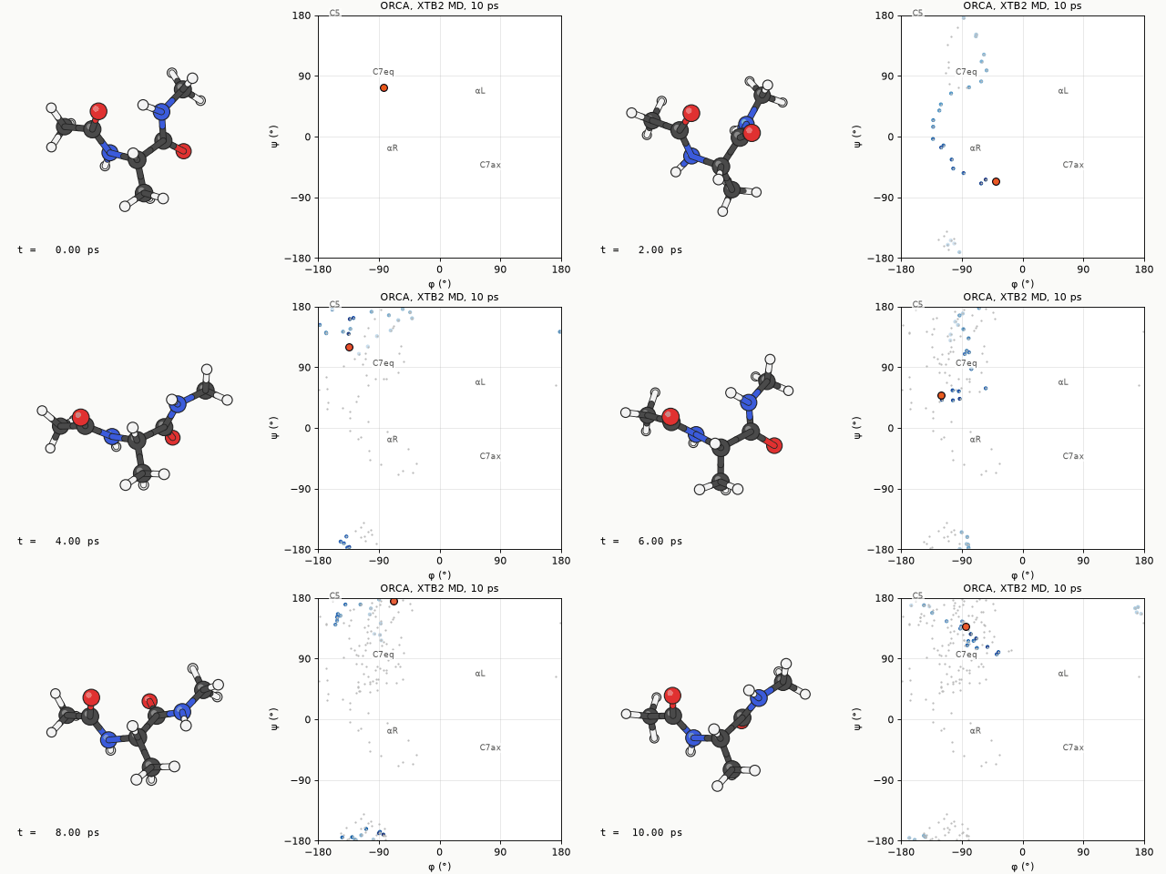
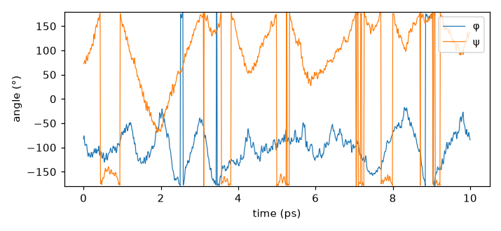
The molecule starts in C7eq (ψ ≈ 50–100°) and makes five round trips between C7eq and the C5/β region over the 10 ps. In the C5/β region ψ sits near ±180°, which is where the ψ line in the plot above jumps between the top and bottom edges. Between 1.6 and 2.3 ps ψ drops to −69° and briefly visits the αR side. Binned by ψ alone, 52% of the frames are C5/β, 42% C7eq and 7% αR. φ, on the other hand, stays between −50° and −180° throughout and never crosses to the positive-φ αL and C7ax regions. The 28 frames where φ reads +164° to +180° are just values wrapped across the −180° boundary. That barrier is hard to cross in 10 ps at 300 K; metadynamics is the tool for it.
The initial velocities were drawn at 300 K, but because the structure started at a minimum, part of the kinetic energy went straight into potential energy and the temperature fell to 112 K within 8 fs. The NHC thermostat then fed energy back in: after discarding the first 1 ps, the mean was 301.6 ± 63.7 K (standard deviation), and 1 ps block averages ranged from 275 to 322 K. For a 22-atom molecule the instantaneous temperature fluctuates this much even in a canonical ensemble; the expected value for 60 degrees of freedom is 300 K × √(2/60) ≈ 55 K. The conserved quantity, which includes the thermostat, drifted by only 2 × 10⁻⁵ Eh (0.01 kcal/mol) over 10 ps, so the 0.5 fs step was small enough. See the o03 input, o03 output, and o03-xtb-md.md.log with the temperature and energies at every step.
The trajectory is plain xyz, so a few lines of Python extract the dihedrals.
import numpy as np

def dihedral(x, i, j, k, l):
    b0, b1, b2 = x[i] - x[j], x[k] - x[j], x[l] - x[k]
    b1 /= np.linalg.norm(b1)
    v = b0 - b0 @ b1 * b1
    w = b2 - b2 @ b1 * b1
    return np.degrees(np.arctan2(np.cross(b1, v) @ w, v @ w))

# atoms count from 0; for this molecule φ = (1, 3, 4, 6), ψ = (3, 4, 6, 8)
Cost by method
The same molecule and input were run for 200 steps (100 fs) with the forces switched to r2SCAN-3c, and the time per step compared.
| Method | Time per step (8 cores) | Time for 10 ps |
|---|---|---|
| GFN2-xTB / ALPB | 0.173 s | 57 min 48 s (measured) |
| r2SCAN-3c / CPCM | 18.6 s (200 steps in 3711 s) | about 103 h (estimated) |
That is roughly a factor of 107 per step. In 1 h 2 min, about the time xTB needed for 10 ps, r2SCAN-3c covered only
100 fs. Over those 100 fs the temperature, again starting from a minimum, fell to 115 K within 7.5 fs and averaged only
174 K over the last 50 fs. The trajectory is far from equilibrium, so it says nothing about structure; it was used only
to measure the cost per step (o04 input ·
o04 output ·
o04-r2scan-md.md.log). Of the 57 min 48 s for xTB, 51 min 17 s (89%) was spent inside xtb and about
5 minutes (9%) in what the MD module reports separately as "dark time": ORCA starting otool_xtb as a new
process at every step and exchanging files with it. For a molecule this small, that overhead is a noticeable share.
DFT MD is for short reactive events or for checking xTB results; long runs that sweep conformational space are done with xTB.
Splitting long runs
The MD module rewrites basename.mdrestart at every step. If a job is cut off by the cluster's time limit,
resubmitting the same input continues the run. With the two lines below placed just before Run, the first
run and every continuation use the same input.
%md
   Timestep   0.5_fs
   Thermostat NHC 300_K Timecon 50.0_fs
   Dump Position Stride 20 Filename "traj.xyz"
   Restart    IfExists             # read the restart file only if it exists
   Initvel    300_K No_Overwrite    # skip if velocities are already known
   Run        20000
endOnly positions, velocities, the NHC internal state, metadynamics hills and the step counters. Thermostat, dump and constraint settings are not stored, so keep them in the input.
Metadynamics
Plain MD often fails to cross barriers of only a few kcal/mol within tens of picoseconds. Metadynamics piles Gaussian hills where the system has already been, pushing it elsewhere, and reconstructs the free-energy surface from the accumulated hills. With φ and ψ as collective variables:
%md
   ...
   Manage_Colvar Define 1 Dihedral Atom 1 Atom 3 Atom 4 Atom 6   # φ
   Manage_Colvar Define 2 Dihedral Atom 3 Atom 4 Atom 6 Atom 8   # ψ
   Metadynamics Colvar 1 Scale 10.0_Deg Colvar 2 Scale 10.0_Deg
   Metadynamics HillSpawn 40 0.5 1.0 Store 2000
   Run        100000
end
The three HillSpawn values are how many steps between hills, the hill height (kJ/mol) and the width (in
Scale units). A roughly converged free-energy surface usually takes several tens of thousands of steps.
For this guide the metadynamics of the same molecule was run with the standalone xtb program; the results are in the
xtb guide.
When to use ORCA MD
- ORCA MD fits: short dynamics that need DFT-level or better forces, QM/MM dynamics, or runs chained with other ORCA features in one input.
- Standalone xtb is easier: long conformational sampling where xTB is enough. SHAKE allows larger time steps, and it feeds straight into CREST.
- Periodic systems: solids, surfaces and explicit solvent boxes belong in Quantum ESPRESSO or force-field LAMMPS.
The MD module was developed by Martin Brehm. The MD section of the ORCA manual lists the references to cite.