Inside periodic boundary conditions, a surface is modeled as a slab: a few atomic layers plus a vacuum layer. Adsorption energies, surface energies, and work functions all start here.
Building slabs: never by hand
Writing slab coordinates by hand is an error factory. Use a generator such as ASE or pymatgen.
from ase.build import surface, bulk
from ase.io import write

feo = bulk('FeO', 'rocksalt', a=4.33)
slab = surface(feo, (1, 0, 0), layers=4, vacuum=8.0)   # 8 Å vacuum each side
slab.center(axis=2)
write('feo100.scf.in', slab, format='espresso-in',
      pseudopotentials={'Fe': 'Fe.pbe-spn-kjpaw_psl.1.0.0.UPF',
                        'O':  'O.pbe-n-kjpaw_psl.1.0.0.UPF'},
      kpts=(6, 6, 1),                                   # 1 along the vacuum
      input_data={'system': {'ecutwfc': 70, 'ecutrho': 700,
                             'occupations': 'smearing', 'degauss': 0.01}})
Open the generated file and read the CELL_PARAMETERS and
ATOMIC_POSITIONS yourself. Being able to read generator output is what
Chapter 03 was for.
A note on magnetism: a 1×1 (100) cell cannot geometrically hold the
AFM-II order of FeO (alternating (111) spin planes), which is why this demo
is nonmagnetic. Real magnetic-surface work needs a larger cell that fits
the ordering, plus starting_magnetization seeds.
Slab conventions:
- One k-point along the vacuum direction (there is no dispersion there).
- Pin the bottom one or two layers at bulk positions (
if_pos 0 0 0) and relax the top. - For cell optimization use
cell_dofree='2Dxy'to freeze the vacuum direction. - Vacuum thickness and layer count are themselves convergence parameters.
The dipole correction
An asymmetric slab (adsorbate or reconstruction on one face) builds a potential difference across the cell, and the periodic images then impose a spurious electric field. The dipole correction cancels it with a sawtooth potential.
&CONTROL
  ...
  tefield   = .true.     ! the two switches live in &CONTROL
  dipfield  = .true.
/
&SYSTEM
  ...
  edir      = 3          ! along z
  emaxpos   = 0.90       ! middle of the vacuum (fractional)
  eopreg    = 0.05
  eamp      = 0.0        ! correction only, no external field
/
Mind the namelist assignment: tefield and dipfield belong to
&CONTROL, while edir, emaxpos, eopreg, eamp belong to
&SYSTEM. Putting tefield into &SYSTEM stops the run immediately with
read_namelists ... bad line (measured; tutorials get this wrong
regularly). And emaxpos, the sawtooth peak, must sit inside the
vacuum; letting it cross the slab produces nonsense.
The work function
$$\Phi = V_{\mathrm{vacuum}} - E_F$$
Procedure: SCF, then pp.x with plot_num=11 (bare + Hartree potential),
then a planar average parallel to the surface (average.x or your own
parser), then subtract the Fermi level from the flat vacuum plateau.
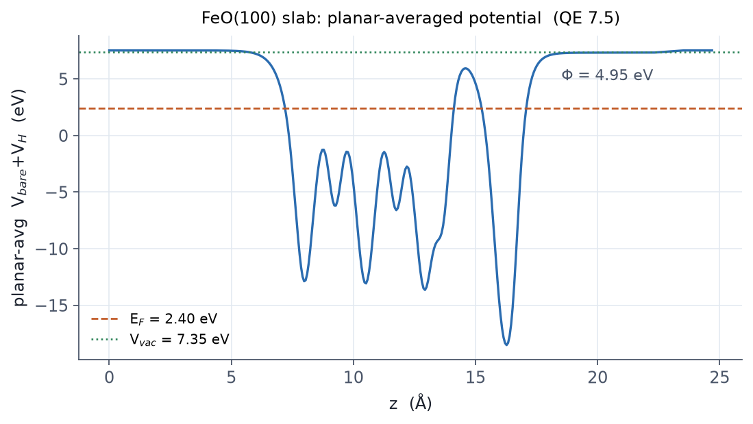
If the slab energy is sensitive to the vacuum thickness, dipole
interactions survive: enable dipfield and add vacuum. If
the planar-averaged potential does not flatten in the vacuum (a slope
remains), the correction position (emaxpos) is wrong or
the vacuum is too thin. Read the work function only after you
have seen the vacuum plateau flatten.
Related examples
- E13 · Slabs and AIMD: generation, relaxation, and a measured work function.
- E9 / E10: the bulk references to compute before any slab.