Goal
Three applications in one pass: (1) generate a FeO(100) slab with ASE
(never by hand), (2) relax it with the dipole correction on and extract the
work function with pp.x, and (3) run Born-Oppenheimer MD on the
bulk FeO cell as the starting point for sampling ML training data.
Background in Chapter 15 and
Chapter 16.
New here
| Item | Role |
|---|---|
ase.build.surface |
The slab generator; no hand-written coordinates |
tefield/dipfield/edir/emaxpos |
The dipole correction |
FixAtoms → if_pos 0 0 0 |
Pinning the bottom layers |
calculation='md' + SVR |
BOMD with a thermostat |
pp.x plot_num=11 |
The electrostatic potential for the work function |
Input files
gen_slab.py · feo_md.in · pp_workfunction.in
The generator in full:
"""Generate a FeO(100) slab and write it as a QE input.
Never write slab coordinates by hand; always use a generator."""
from ase.build import bulk, surface
from ase.io import write
from ase.constraints import FixAtoms

# rocksalt FeO with the cubic lattice constant a = 4.33 A
feo = bulk("FeO", "rocksalt", a=4.33)

# cut a (100) surface: 4 layers, 8 A of vacuum added on each side
# (16 A total once the cell is closed), then center the slab in the cell
slab = surface(feo, (1, 0, 0), layers=4, vacuum=8.0)
slab.center(axis=2)

# pin the bottom half of the layers at bulk positions; ASE constraints are
# translated into QE if_pos flags (0 0 0 on the fixed atoms)
zs = sorted(set(round(z, 3) for z in slab.positions[:, 2]))
fixed_z = set(zs[: len(zs) // 2])
slab.set_constraint(FixAtoms(
    indices=[i for i, a in enumerate(slab) if round(a.position[2], 3) in fixed_z]))

write(
    "feo100.scf.in", slab, format="espresso-in",
    pseudopotentials={"Fe": "Fe.pbe-spn-kjpaw_psl.1.0.0.UPF",
                      "O":  "O.pbe-n-kjpaw_psl.1.0.0.UPF"},
    kpts=(6, 6, 1),          # one k-point along the vacuum direction
    input_data={
        # tefield/dipfield are &CONTROL variables (&SYSTEM placement raises
        # read_namelists); they switch on the sawtooth dipole correction
        "control": {"calculation": "relax", "prefix": "feo100",
                    "outdir": "./tmp/", "pseudo_dir": "./pseudo/",
                    "tprnfor": True, "forc_conv_thr": 1.0e-4,
                    "tefield": True, "dipfield": True},
        # nonmagnetic demo: a 1x1 (100) cell cannot hold the AFM-II order.
        # edir=3: correction along z; emaxpos=0.90 puts the sawtooth peak in
        # the middle of the vacuum; eamp=0 means correction only, no field
        "system": {"ecutwfc": 70, "ecutrho": 700,
                   "occupations": "smearing", "smearing": "mv", "degauss": 0.01,
                   "edir": 3, "emaxpos": 0.90, "eopreg": 0.05, "eamp": 0.0},
        # slabs with vacuum are inhomogeneous: gentle mixing + local-TF,
        # and more than the default 100 iterations for the first SCF
        "electrons": {"conv_thr": 1.0e-8, "mixing_beta": 0.2,
                      "mixing_mode": "local-TF", "electron_maxstep": 200},
        "ions": {"ion_dynamics": "bfgs"},
    },
)
print("wrote feo100.scf.in; open it and read CELL_PARAMETERS/ATOMIC_POSITIONS yourself")
Open the generated feo100.scf.in and read it yourself: the
CELL_PARAMETERS, the ATOMIC_POSITIONS (angstrom), the if_pos flags.
Being able to read generator output is what
E2 was for. The slab SCF is nonmagnetic by design:
a 1×1 (100) cell cannot geometrically hold the AFM-II order of FeO
(Chapter 15).
The MD deck, fully annotated (the same FeO(+U) bulk cell as E11):
! E13: Born-Oppenheimer MD on the bulk FeO(+U) cell.
! dt is in Rydberg atomic units: 20.0 a.u. = 0.968 fs

&CONTROL
  calculation = 'md'
  prefix      = 'feo_md'
  outdir      = './tmp/'
  pseudo_dir  = './pseudo/'
  nstep       = 2000         ! 2000 steps x 0.968 fs ~ 1.9 ps
  dt          = 20.0         ! TIME STEP IN RYDBERG A.U., not femtoseconds
  tprnfor     = .true.       ! forces on every step: that is the training data
  tstress     = .false.      ! Hubbard stress dies with stres_hub under nosym+U (measured);
                             ! recompute stress on extracted frames with scf runs if needed
  disk_io     = 'none'       ! do not write wavefunctions every step: I/O kills MD
/
&SYSTEM
  ...                        ! same cell/cutoffs/magnetization as E11, plus:
  nosym       = .true.       ! mandatory for MD: thermal motion breaks the initial
                             ! symmetry in step 1 (checkallsym error without this)
/
&ELECTRONS
  conv_thr    = 1.0d-6       ! BOMD-level threshold; nosym+U struggles below this (measured)
  mixing_beta = 0.2
  mixing_mode = 'local-TF'
  electron_maxstep = 300
  mixing_fixed_ns  = 30      ! freeze the DFT+U ns matrix for the first 30 iterations:
                             ! without symmetry the degenerate t2g orbitals rotate freely
                             ! and the SCF stalls otherwise (measured)
/
&IONS
  ion_dynamics    = 'verlet' ! velocity-Verlet integrator
  ion_temperature = 'svr'    ! stochastic velocity rescaling thermostat (canonical sampling)
  tempw           = 300.0    ! target temperature in K
  nraise          = 100      ! thermostat coupling period, in steps (~0.1 ps here)
/
And the work-function extraction:
! extract the electrostatic potential of the relaxed slab.
! two namelists: WHAT to extract, then HOW to write it.
&INPUTPP
  prefix   = 'feo100'          ! the slab relaxation's prefix
  outdir   = './tmp/'
  filplot  = 'feo100.pot.dat'  ! intermediate file
  plot_num = 11                ! 11 = bare + Hartree potential (no XC), the
                               ! standard choice for vacuum-level alignment
/
&PLOT
  nfile         = 1
  filepp(1)     = 'feo100.pot.dat'
  weight(1)     = 1.0
  iflag         = 3            ! 3 = full 3D grid
  output_format = 6            ! 6 = Gaussian cube
  fileout       = 'feo100.pot.cube'
/
! afterwards: planar-average the cube over x,y, check the vacuum plateau is
! FLAT, then work function = V_vacuum - E_Fermi
Run
python gen_slab.py                                     # writes feo100.scf.in
mpirun -np 8 pw.x -nk 4 -in feo100.scf.in > feo100.relax.out
mpirun -np 8 pp.x -in pp_workfunction.in  > pp_workfunction.out
mpirun -np 8 pw.x -nk 4 -in feo_md.in     > feo_md.out
For the measurements we capped the relaxation at 25 BFGS steps and ran the
MD on an nstep=200 copy (about 0.2 ps); the distributed input keeps the
original nstep=2000. Along the way we found and fixed several defects in
the original decks (the tefield/dipfield namelist placement, the
missing nosym and mixing_fixed_ns for MD; see the common-mistakes box).
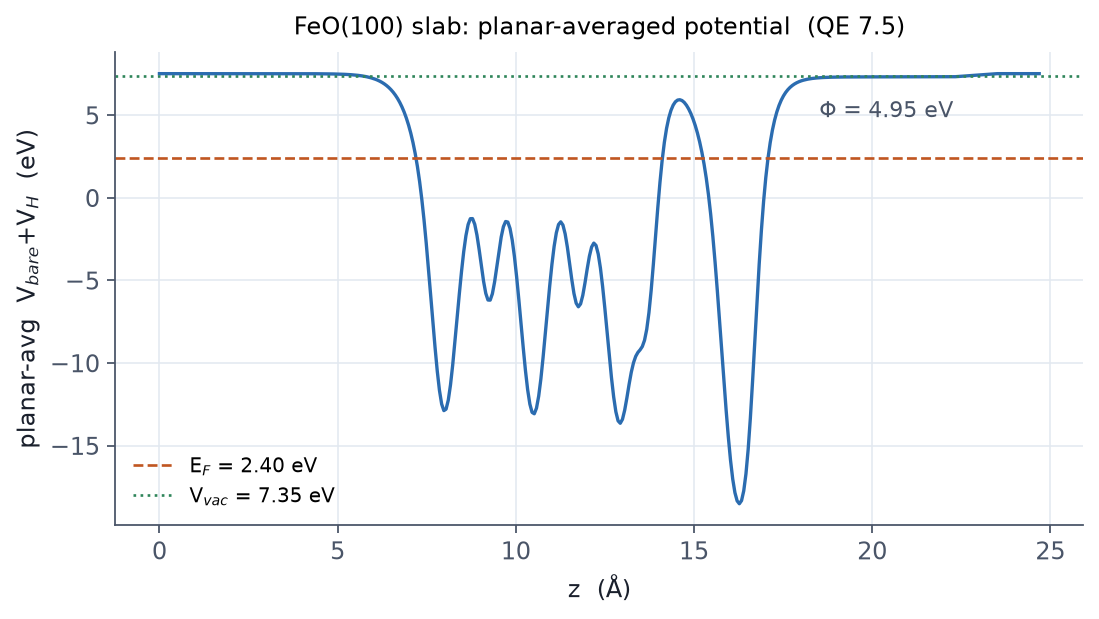
Output and figure: measured (1) slab and work function
| Item | Measured (QE 7.5) |
|---|---|
| Slab | FeO(100), 4 layers, 8 atoms (1×1), 16 Å vacuum, nonmagnetic demo |
| Relaxation | 25-step BFGS copy (final total force 0.005 Ry/au: a partial optimization for the demo) |
| Vacuum level / Fermi level | 7.35 eV / 2.40 eV (vacuum flatness std 0.05 eV) |
| Work function Φ = V_vac − E_F | 4.95 eV |
Output and figure: measured (2) BOMD
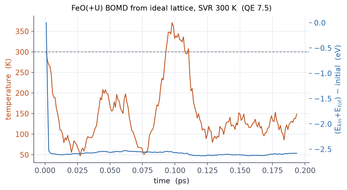
That early transient is itself the practical lesson: extract training frames only after equilibration. Mixing the transient into a dataset contaminates it with artificially high-energy structures.
Principles for ML datasets (Chapter 16): identical cutoffs, k-grid, smearing and U on every frame; converge on forces; subsample (every 50 steps or so) against frame correlation; and if you need stress, compute it in separate scf runs on the extracted frames (see the box).
Exercises
- Rebuild with
layers=4 → 6and see how the work function moves (layer count is a convergence parameter too). - Turn
dipfieldoff and watch the vacuum region of the planar average acquire a slope. - Write a parser that pulls energy and force frames from the MD log every 50 steps.
- Recompute one frame at 60 and 90 Ry cutoffs and compare the forces against your ML accuracy target (~50 meV/Å).
tefield/dipfield belong to
&CONTROL. Put them in &SYSTEM
and the run dies instantly with
read_namelists ... bad line (only the position parameters
edir etc. are &SYSTEM variables); we hit this and
fixed the generator.
MD requires nosym=.true.: thermal motion
breaks the initial symmetry in the first step, and without it the run
stops at checkallsym.
DFT+U with nosym stalls the SCF: rotations among the
degenerate t2g orbitals keep the density sloshing (stuck at 7×10⁻⁵ Ry
after 100 iterations); mixing_fixed_ns=30 (freeze the ns
matrix for the first iterations) releases it, after which even 10⁻⁸ is
hard to reach, so the distributed input uses the BOMD-conventional
conv_thr = 1.0d-6.
Hubbard stress dies under nosym: with
tstress=.true. the run aborts at
stres_hub: non-symmetric stress contribution; NVT sampling
does not need stress, so it is off, and stress for training data comes
from separate scf runs on extracted frames. Finally, emaxpos
(the sawtooth peak) must sit in the middle of the vacuum, and
dt is in Rydberg atomic units (20 a.u. ≈ 0.968 fs);
read it as femtoseconds and the trajectory explodes at once.
Related chapters
15 Surfaces, slabs, work function · 16 Molecular dynamics · 11 Densities and potentials